Why convolutions?

Preface #

Many a times engineers have had the ideas of convolutions lazily puked on them during a class on signal theory. Rarely is it properly explained what convolutions mean, how they relate to impulse responses and how all the pieces fall together.

I think signal theory is one of the most interesting topics learnt in electrical engineering. In a way, it is far more abstract and more mathematical than much of what else is learnt. However, it is also a topic that is very easily applicable to the behaviour of everyday objects. It’s easy to appreciate signal theory even if your background isn’t electrical engineering but mechanical engineering, physics, computer science etc. It also serves as a precursor to some very interesting fields. It goes hand in hand with control theory, information theory and so on and can give some great insights into computer vision (what are images but discretised 2D signals?). Anyways, lets dive in!

From the bottom #

Signal theory concerns itself with the idea of signals, essentially time-varying (or space-varying) functions, in particular ones that go through systems.

We may see signals and the systems they go through in many ways. Maybe it’s an electrical signal representing the music playing in our earphones, or the input force due to wind on a bridge, or the even digital images that we put through filters on our phones. The essential idea is that the system takes the input and “transforms” it into the output signal. Said another way, the system “responds” to the input signal a certain way, which we measure as the output of the system.

LTI systems #

Now systems we encounter in reality are not magic. They are governed by physical laws and design principles which means they follow some set rules which describe how an input is transformed into the output. That means we can characterise and study systems and their behaviour in an effort to predict how they behave under certain inputs, which as you imagine, can be very useful.

Not all systems are easy to characterise however. So at least at first, we try to focus on systems we can understand. In particular, we love what are called Linear Time-Invariant Systems, or LTI systems. LTI systems obey two properties that make them much nicer to study. In particular:

• They are linear - If you send two different inputs into the system and add their outputs together, the result is the same as adding the two inputs and sending it through the system. You can also think of it as similar to a function that obeys the principle of superposition, or a function \(f(x(t))\) such that $$f(x_1(t)) + f(x_2(t)) = f(x_1(t) + x_2(t))$$ and homogeniety, or $$f(ax(t))=af(x(t))$$ As Feynman puts it, linear systems are important because we can solve them! About half the time, we’re solving linear systems and the other half, we’re trying to approximate non-linear systems as linear systems to understand them.
• They are time-invariant - Your system isn’t sensitive to what time you send the input. Sending the input at a different time doesn’t fundamentally change how the system reacts to it. In other terms, if \(x(t)\) is the input and the output is \(x’(t)\), then the output due to \(x(t-\Delta t)\) is \(x’(t-\Delta t)\)

There are many systems in reality that are LTI. There are even more systems that are behave LTI to certain extents and thus can be approximated as such.

Impulse response #

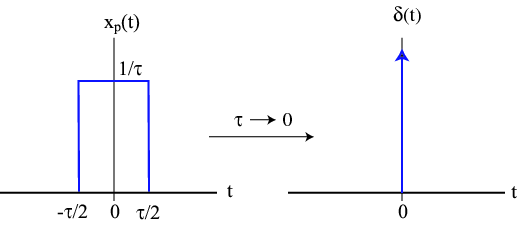
Now we’re going to take a detour for a bit and see how this connects back. Let is think about what happens when we send an “impulse” signal to the system. By impulse, we mean a very sharp instantaneous pulse in the input. Physicists might know this as the Dirac delta. Engineers generally call it the impulse function.

Now we may ponder what happens when we send that impulse as an input to an LTI system. We will get a response back, an output, which we’re going to call our impulse response. I am going to call this impulse response \(h(t)\). Now let us consider another input, this time consisting of multiple impulses. at different times i.e. \(x(t)=\delta(t) + 2\delta(t-1)\). Now since we know that the system is LTI, so hence from our earlier observations about time invariance and linearity, we can conclude the output for this new input will be \(h(t)+2h(t-1)\). Simple, right?

The Convolution #

Now let us consider that we were able to write an arbitrary input as a sum of many impulse inputs. It would be so simple to find out the output response as a scaled sum of a bunch of impulse responses. Well, that’s essentially exactly what we do!

I think it’s easiest to see how a convolution arises when viewing things in the discrete case. In the discrete case, an impulse input is simply:

delta[t] = 1 0 0 0 0 0 ...

Now say when we send in that impulse to our system, we get an impulse response like so

h[t] = 3 2 1 0 0 0 ...

If our input was now

x[t] = 2 1 0 0 0 0 ...

We could write it as

f[x[t]] = 2*h[t] + h[t-1]
        = 6 4 2 0 0 0 ...
        + 0 3 2 1 0 0 0 ...
        -------------------
        = 6 7 4 1 0 0 0 ...

Did you see that? We were able to predict a non-impulse input’s response by just expressing it as a sum of impulses. In particular, we can generalise this to $$ f[x[t]] = \sum_{m=0}^{\infty} x[m]h[t-m]$$ Where our output is being given by a sum of many delayed and scaled impulse responses based on the values of the inputs. In fact, this is a convolution! This is a discrete convolution, one you may be familiar with from Digital Signal Processing or a Deep Learning class. The only difference being that here we choose to start off with time \(t=0\) while generally we can start off with \(t=-\infty\).

Our convolution in the continuous state is just the continuation of that, where a sum is replaced with an integral and now we’re summing infinite very small impulse responses! $$ f(x(t)) = (f * h)(t) = \int_{-\infty}^{\infty} x(\tau)h(t-\tau), d\tau $$

If you squint and look closely, you can sort of begin to see how the properties of linearity and time invariance in a signal can lead to convolutions with the impulse response of LTI systems being fundamental in describing the behaviour with arbitrary inputs!

What’s next? #

Once we justify why convolutions work in characterising the behaviour of LTI systems, we start to realise convolutions are hard to calculate and that it is difficult to talk about systems in this manner. But what saves us is a theorem aptly named the convolution theorem. The convolution theorem becomes a ground shaker because it links the convolution operation in the time domain with simple multiplication in the Laplace or Fourier domain. This is due to the fact that sinuisoids are eigenfunctions of LTI systems and it leads to interesting avenues where we are able to study our LTI systems in a domain where we can characterise their behaviour in a more geometric manner through the scaling it causes on the Laplace domain. But all of that is readily taught in undergraduate engineering courses and a story for another time…